Tutorial
Basics
A brief tutorial of a Laval rotor should show the working principle of AMrotor for building a rotordynamic model, followed by examples referring to the available analysis methods. More advanced models can be found under Examples.
To run a simulation with AMrotor, two scripts are required:
Configuration script, contains parameters with information about the rotor and all additional components. These parameters are processed in the subsequent Simulation script.
Simulation script, contains the composition of the model and the definition of desired analysis methods that are applied to the model.
How to build a model?
The scope of this tutorial is to build a simple Laval rotor model with two simple radial bearings and a disk in the middle, which is modeled as part of the rotor (no additional disk component).
Configuration script
The following Config script can be inserted into an empty Matlab script by copy and paste. The script must then be saved in the AMrotor path. For this tutorial we save the script under the name “Config_Tutorial” in the Simulation(Simulations)-folder of AMrotor. It may be necessary to add the folder explicitly to the path. The name of the Configuration script is important, because it will be used later in the Simulation script.
For this simple example not all components (only rotor and bearings) are necessary, but it is important that all components (sensors, pid controllers, active magnetic bearings, …) are initialized to avoid errors.
 1 %% Configuration
 2
 3 %% ================Rotor===================================================
 4 %% Building of the rotor struct
 5 cnfg.cnfg_rotor.name = 'Simple example: Laval-Rotor';
 6 % All units in SI
 7 cnfg.cnfg_rotor.material.name = 'steel';
 8 cnfg.cnfg_rotor.material.e_module = 211e9;  %[N/m^2]
 9 cnfg.cnfg_rotor.material.density  = 7860;   %[kg/m^3]
10 cnfg.cnfg_rotor.material.poisson  = 0.3;    %[-]
11 % Rayleigh damping: D=alpha1*K + alpha2*M
12 cnfg.cnfg_rotor.material.damping.rayleigh_alpha1= 1e-5;
13 cnfg.cnfg_rotor.material.damping.rayleigh_alpha2= 10;
14
15 %% Rotor Config
16 rW = 10e-3; % Radius of the shaft [m]
17 rS = 50e-3; % Radius of the disc [m]
18 % Format of the geometry definition: {[z, r_outer, r_inner], ...} without..
19 % start- and end-node
20 cnfg.cnfg_rotor.geo_nodes = {[0 rW 0], [0.220 rW 0], [0.220 rS 0], ...
21 [0.280 rS 0], [0.280 rW 0], [0.500 rW 0]};
22 clear rW rS
23
24 %% FEM Config
25 cnfg.cnfg_rotor.mesh_opt.name = 'Mesh 1';
26 % Number of refinement steps between d_min and d_max
27 cnfg.cnfg_rotor.mesh_opt.n_refinement = 10;
28 cnfg.cnfg_rotor.mesh_opt.d_min = 0.001;
29 cnfg.cnfg_rotor.mesh_opt.d_max = 0.05;
30 % Definition of the element radius, if the geometry radius is not ...
31 % constant in this section. Options: symmetric, mean, upper sum, lower sum
32 cnfg.cnfg_rotor.mesh_opt.approx = 'symmetric';
33
34 %% ====================Sensors============================================
35 %% Initialization of the sensor section in the struct
36 cnfg.cnfg_sensor=[];
37 count = 0;
38
39 %% =========================Components====================================
40 %% Initialization of the components section in the struct
41 count = 0;
42 cnfg.cnfg_component = [];
43
44 %% Bearings
45 count = count + 1;
46 cnfg.cnfg_component(count).name = 'RadBearing1';
47 cnfg.cnfg_component(count).type='Bearings';
48 cnfg.cnfg_component(count).subtype='SimpleBearing';
49 cnfg.cnfg_component(count).position=0e-3; % [m]
50 cnfg.cnfg_component(count).stiffness=1e6; % [N/m]
51 cnfg.cnfg_component(count).damping = 0; % [Ns/m]
52 count = count + 1;
53 cnfg.cnfg_component(count).name = 'RadBearing2';
54 cnfg.cnfg_component(count).type='Bearings';
55 cnfg.cnfg_component(count).subtype='SimpleBearing';
56 cnfg.cnfg_component(count).position=500e-3; % [m]
57 cnfg.cnfg_component(count).stiffness=1e6; % [N/m]
58 cnfg.cnfg_component(count).damping = 0; % [Ns/m]
59
60 %% =========================Loads=========================================
61 %% Initialization of the load section in the struct
62 cnfg.cnfg_load=[];
63 count = 0;
64
65 %% ========================PID-controller==================================
66 %% Initialization of the pid-controller section in the struct
67 cnfg.cnfg_pid_controller=[];
68 count = 0;
69
70 %% ======================Active Magnetic Bearing===========================
71 %% Initialization of the active magnetic bearing section in the struct
72 cnfg.cnfg_activeMagneticBearing = [];
73 count = 0;
By executing the saved script the Config-struct (cnfg) will be created.
Simulation script
After setting up the Configuration script, the Simulation script must be created. The following part of the Simulation script contains the assembly and visualization of the model and can be inserted into an empty Matlab script by copy and paste. The Simulation script can be saved in the same folder as the corresponding Configuration script. For this tutorial it is important that the name of the called Configuration script in the Simulation script is equal to “Config_Tutorial” (line 9).
1 %% Simulation
2 %% Clean up
3 close all
4 clear all
5 % clc
6
7 %% Import and formating of the figures
8 import AMrotorSIM.*; % path
9 Config_Tutorial; % Corresponding cnfg-file
10 Janitor = AMrotorTools.PlotJanitor(); % Instantiation of class PlotJanitor
11 Janitor.setLayout(2,3); %Setting layout of the figures
12
13 %% Assembly of the rotordynamic model
14 r=Rotorsystem(cnfg,'Laval-Rotor'); % Instantiation of class Rotorsystem
15 r.assemble; % Assembly of the model parts, considering the ...
16 % components (sensors,..) from the cnfg-file
17 r.rotor.assemble_fem; % assembly of the global (rotor) system ...
18 % matrices: M, D, G, K
19
20 %% Visualization of the assembled rotor model
21 r.show; % lists the associated components of the model in teh Matlab ...
22 % Command Window
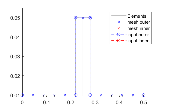
23 r.rotor.show_2D(); % Plot of a side view of the rotor elements
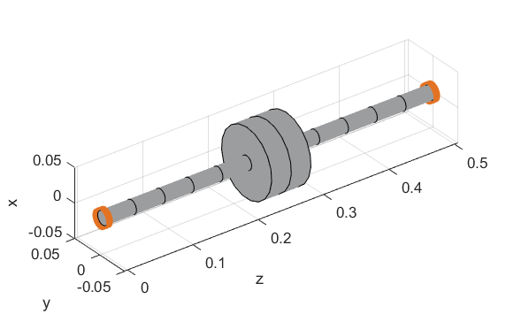
24 g=Graphs.Visu_Rotorsystem(r); % Instantiation of class Visu_Rotorsystem
25 g.show(); % Plot of a 3D-isometry of the rotor with sensors, loads,...
26 Janitor.cleanFigures(); % Formatting of the figures
After executing the Simulation script the following figures of the rotor model appear:
More advanced examples including subsequent analysis methods can be found under Examples.
How to make a Campbell analysis?
Note
The following analysis method does not work with the previous example How to build a model?, because in that minimal example some components (e.g. sensors, loads, …) are missing. To merge a model with an analysis method see Examples.
In general, the analysis methods are defined in the Simulation script and can be divided into two sub-blocks:
Calculation code block
Visualization code block
To calculate and visualize a Campbell analysis, the following code is required in the Simulation script after the lines of code for assembling the model.
 1 %% Calculation
 2 cmp = Experiments.Campbell(r); % Instantiation of class Campbell for calculation
 3 cmp.set_up(0:2e2:2e3,20); % Set up (omega range in 1/min, #modes)
 4 cmp.calculate(); % Calculation
 5
 6 %% Visualization
 7 cmpDiagramm = Graphs.Campbell(cmp); % Instantiation of class Campbell for visualization
 8                             % of the obtained results
 9 cmpDiagramm.print_damping_zero_crossing(); % Prints in the Command Window
10 cmpDiagramm.print_critical_speeds() % Prints in the Command Window
11 cmpDiagramm.set_plots('all'); % Plots the visualization (Figures)
12 Janitor.cleanFigures(); % Formatting of the figures
How to make a Modal analysis?
Note
The following analysis method does not work with the previous example How to build a model?, because in that minimal example some components (e.g. sensors, loads, …) are missing. To merge a model with an analysis method see Examples.
In general, the analysis methods are defined in the Simulation script and can be divided into two sub-blocks:
Calculation code block
Visualization code block
To calculate and visualize a Modal analysis, the following code is required in the Simulation script after the lines of code for assembling the model.
 1 %% Calculation
 2 m=Experiments.Modalanalyse(r); % Instantiation of class Modalanalyse for calculation
 3 m.calculate_rotorsystem(16,0); % Calculation (#modes, rotation speed)
 4
 5 %% Visualization
 6 esf= Graphs.Eigenschwingformen(m); % Instantiation of class Eigenschwingformen for
 7                             % visualization of the obtained results
 8 esf.print_frequencies(); % Prints EF in the Command Window
 9 esf.plot_displacements(); % Plots the 2D mode shapes
10 % esf.set_plots('half','Overlay'); % Plots of the odd-numbered eigenmodes ..
11                             % in overlay with the original rotor
12 esf.set_plots(10,'Overlay','Skip',5,'tangentialPoints',30,'scale',3); % ...
13                             % Plot of the 3D mode shapes
14 Janitor.cleanFigures(); % Formatting of the figures
How to make a Stationary time integration?
Note
The following analysis method does not work with the previous example How to build a model?, because in that minimal example some components (e.g. sensors, loads, …) are missing. To merge a model with an analysis method see Examples.
In general, the analysis methods are defined in the Simulation script and can be divided into two sub-blocks:
Calculation code block
Visualization code block
To calculate and visualize a Stationary time integration, the following code is required in the Simulation script after the lines of code for assembling the model. In a Stationary time integration, the angular velocity of the rotor is kept at a constant value.
 1 %% Calculation
 2 St_Lsg = Experiments.Stationaere_Lsg(r,[500],[0:0.001:0.025]); % In...
 3     %stantiation of class Stationaere_Lsg
 4 St_Lsg.compute_ode15s_ss; % ode15s - method
 5 %St_Lsg.compute_newmark; % newmark - method
 6
 7 %% Visualization
 8 t = Graphs.TimeSignal(r, St_Lsg); % Instantiation of class TimeSignal
 9 o = Graphs.Orbitdarstellung(r, St_Lsg); % Instantiation of class ...
10                                  % Orbitdarstellung
11 f = Graphs.Fourierdarstellung(r, St_Lsg); % Instantiation of class ...
12                                    % Fourierdarstellung
13 fo = Graphs.Fourierorbitdarstellung(r, St_Lsg); % Instantiation of class ..
14                                          % Fourierorbitdarstellung
15 w = Graphs.Waterfalldiagramm(r, St_Lsg); % Instantiation of class ...
16                                   % Waterfalldiagramm
17 w2 = Graphs.WaterfalldiagrammTwoSided(r, St_Lsg); % Instantiation of ...
18                                    % class WaterfalldiagrammTwoSided
19 for sensor = r.sensors % Loop over all sensors for plotting the sensor results
20       t.plot(sensor); % Time signal
21       o.plot(sensor); % Orbits
22       f.plot(sensor); % Fourier
23       fo.plot(sensor,1); % Fourierorbit 1st order
24       fo.plot(sensor,2); % Fourierorbit 2nd order
25       w.plot(sensor); % Waterfall
26       w2.plot(sensor); % Waterfall 2sided
27      Janitor.cleanFigures(); % Formatting of the figures
28 end
How to make a Run-up time integration?
Note
The following analysis method does not work with the previous example How to build a model?, because in that minimal example some components (e.g. sensors, loads, …) are missing. To merge a model with an analysis method see Examples.
In general, the analysis methods are defined in the Simulation script and can be divided into two sub-blocks:
Calculation code block
Visualization code block
To calculate and visualize a Run-up time integration, the following code is required in the Simulation script after the lines of code for assembling the model. In a Run-up time integration, the angular velocity of the rotor is linearly variable (up or down) over a defined range.
 1 %% Calculation
 2 Runup = Experiments.Hochlaufanalyse(r,[0,1e3],(0:0.001:0.2)); % In...
 3     %stantiation of class Hochlaufanalyse (Runup)
 4 Runup.compute_ode15s_ss % ode15s - method
 5
 6 %% Visualization
 7 t = Graphs.TimeSignal(r, Runup); % Instantiation of class TimeSignal
 8 o = Graphs.Orbitdarstellung(r, Runup); % Instantiation of class ...
 9                                  % Orbitdarstellung
10 f = Graphs.Fourierdarstellung(r, Runup); % Instantiation of class ...
11                                    % Fourierdarstellung
12 fo = Graphs.Fourierorbitdarstellung(r, Runup); % Instantiation of class ..
13                                          % Fourierorbitdarstellung
14 w = Graphs.Waterfalldiagramm(r, Runup); % Instantiation of class ...
15                                   % Waterfalldiagramm
16 w2 = Graphs.WaterfalldiagrammTwoSided(r, Runup); % Instantiation of ...
17                                    % class WaterfalldiagrammTwoSided
18 for sensor = r.sensors % Loop over all sensors for plotting the sensor results
19       t.plot(sensor); % Time signal
20       o.plot(sensor); % Orbits
21       f.plot(sensor); % Fourier
22       fo.plot(sensor,1); % Fourierorbit 1st order
23       fo.plot(sensor,2); % Fourierorbit 2nd order
24       w.plot(sensor); % Waterfall
25       w2.plot(sensor); % Waterfall 2sided
26      Janitor.cleanFigures(); % Formatting of the figures
27 end
How to get FRF’s from the rotor system?
Note
The following analysis method does not work with the previous example How to build a model?, because in that minimal example some components (e.g. sensors, loads, …) are missing. To merge a model with an analysis method see Examples.
In general, the analysis methods are defined in the Simulation script and can be divided into two sub-blocks:
Calculation code block
Visualization code block
To calculate and visualize frequency response functions (FRF’s), the following code is required in the Simulation script after the lines of code for assembling the model.
 1 %% Calculation
 2 frf=Experiments.Frequenzgangfunktion(r,'FRF'); % Instantiation of ...
 3                     % class Frequenzgangfunktion
 4 type = 'd'; % FRF type: displ. 'd', veloc. 'v', accel. 'a'
 5 inPos = [0,100,200]*1e-3; % Input positions on the rotor axis
 6 outPos = 100e-3; % Output positions along the rotor axis
 7 f = 1:2:100; % Frequency resolution of the FRF
 8 rpm = 0; % Rotational speed
 9 [f,H]=frf.calculate(f,inPos,outPos,type,rpm,{'u_x','u_y','psi_x'}, {'u_x','psi_x'}); % ...
10                   % Calculation of the FRF's from the three input ...
11                   % directions {'u_x','u_y','psi_x'} to the two ...
12                   % output directions {'u_x','psi_x'} at the ...
13                   % corresponding positions
14 [deltaIn,deltaOut]=frf.print_distance_delta; % Plot of the gap between ...
15                   % the desired positions along the rotor axis and ...
16                   % the closest node position in the Command Window.
17 %% Visualization
18 visufrf = Graphs.Frequenzgangfunktion(frf); % Instantiation of ...
19                     % class Frequenzgangfunktion for figures
20 visufrf.set_plots('amplitude','db') % Amplitude plot of all FRF's
21 visufrf.set_plots('phase','db') % Phase plot of all FRF's
22 visufrf.set_plots('bode','log','deg') % Bode plot of all FRF's
23 visufrf.set_plots('nyquist') % Nyquist plot of all FRF's
24 Janitor.cleanFigures(); % Formatting of the figures
How to get FRF’s from time signals of the rotor system?
Note
The following analysis method does not work with the previous example How to build a model?, because in that minimal example some components (e.g. sensors, loads, …) are missing. To merge a model with an analysis method see Examples.
In general, the analysis methods are defined in the Simulation script and can be divided into two sub-blocks:
Calculation code block
Visualization code block
To calculate and visualize frequency response functions (FRF’s) from time signals, the following code is required in the Simulation script after the lines of code for assembling the model. FRF’s from time signals are based on results of previously performed time integrations (see Stationary: How to make a Stationary time integration? or Runup: How to make a Run-up time integration?). It is essential that the desired rotation speed (rpm) for the FRF’s is included in the results from the time integrations performed previously.
 1 %% Calculation
 2 St_Lsg; % Runup; %Results from time integration are necessary (Stationary or Runup)
 3 frf = Experiments.FrequenzgangfunktionTime(St_Lsg); % Instantiation ...
 4                                     % of class FrequenzgangfunktionTime
 5 frf.calculate(r.sensors(2),r.sensors(1),[1100],'u_x','u_x',4,'boxcar'); % Calculation
 6
 7 %% Visualization
 8 visufrf = Graphs.Frequenzgangfunktion(frf); % Instantiation of class FrequenzgangfunktionTime
 9 visufrf.set_plots('bode','log','deg','coh'); % Plot of the FRF's
10 Janitor.cleanFigures(); % Formatting of the figures