MBTR test rig with spring damper elements as bearings
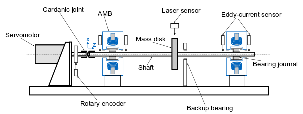
This code example is based on a real magnetic bearing test rig (MBTR). In this MBTR a rotor is mounted on active magnetic bearings (AMB’s). The simulations however uses spring-damper elements to approximate the magnetic bearing behaviour.
Configuration file for the MBTR
This is a Configuration file for a rotor system based on the magnetic bearing test rig (MBTR). The example of the Laval rotor (Simple laval rotor example) serves as a template and has been adapted and extended for the purposes of the MBTR rotor.
The first step is to define the rotor/shaft. This definition can be divided into three parts: Definition of the material parameters, the geometry of the rotor and the properties of the mesh:
Note
In this simulation, not the entire contour of the rotor is included in the rotor geometry. Instead, only the main radius of the rotor and some reinforcements (for transition stiffness purposes) are modeled in the rotor geometry. The other diameter steps of the rotor are later modeled as discs.
 1cnfg.cnfg_rotor.name = 'MBTR - TestRig';
 2cnfg.cnfg_rotor.color = AMrotorTools.TUMColors.TUMGray2; % Rotor color
 3% All units in SI
 4cnfg.cnfg_rotor.material.name = 'steel';
 5cnfg.cnfg_rotor.material.e_module = 211e9; % [N/m^2]
 6cnfg.cnfg_rotor.material.density  = 7860; % [kg/m^3]
 7cnfg.cnfg_rotor.material.poisson  = 0.3; % [-]
 8% Rayleigh damping: D=alpha1*K + alpha2*M
 9cnfg.cnfg_rotor.material.damping.rayleigh_alpha1= 5e-7;
10cnfg.cnfg_rotor.material.damping.rayleigh_alpha2= 0;
11
12%% Rotor Config
13% % Only main shaft radius, shaft steps as disc components
14% raW = 0.004;
15% % Format of the geometry definition: {[z, r_outer, r_inner], ...} ...
16% % without start- and end-node:
17% cnfg.cnfg_rotor.geo_nodes = {[0 0 0], [0 raW 0], [0.702 raW 0]};
18
19% Shaft with reinforcements at the bearing journals and at the disc
20raW = 0.004;
21riW = 0;
22raL = raW*1.2;
23riL = 0;
24raR = raW*1.2;
25riR = 0;
26% Format of the geometry definition: {[z, r_outer, r_inner], ...} without..
27% start- and end-node:
28cnfg.cnfg_rotor.geo_nodes = {[0 0 0], [0 raW riW], [0.094 raW riW], ...
29    [0.094 raL riL], [0.132 raL riL], [0.132 raW riW], ...
30    [0.350 raW riW], [0.350 raR riR], [0.376 raR riR], [0.376 raW riW],...
31    [0.604 raW riW], [0.604 raL riL], [0.642 raL riL], ...
32    [0.642 raW riW], [0.702 raW riW], [0.702 0 0]};
33
34% cnfg.cnfg_rotor.geo_nodes = {[0 0 0], [0 raW riW], [0.094 raW riW], ...
35%                                                      % Shaft
36%     [0.094 raL riL], [0.132 raL riL], [0.132 raW riW], ...
37%                                                      % bearing bushing 1
38%     [0.350 raW riW], [0.350 raR riR], [0.376 raR riR], [0.376 raW riW],...
39%                                                      % Rotor disc
40%     [0.604 raW riW], [0.604 raL riL], [0.642 raL riL], ...
41%                                                      % bearing bushing 2
42%     [0.642 raW riW], [0.702 raW riW], [0.702 0 0]}; % Shaft
43
44%% FEM Config
45cnfg.cnfg_rotor.mesh_opt.name = 'Mesh 1';
46% Number of refinement steps between d_min and d_max:
47cnfg.cnfg_rotor.mesh_opt.n_refinement = 10;
48cnfg.cnfg_rotor.mesh_opt.d_min= 0.002;
49cnfg.cnfg_rotor.mesh_opt.d_max = 0.01;
50% Definition of the element radius, if the geometry radius is not ...
51% constant in this section. Options: symmetric, mean, upper sum, lower sum:
52cnfg.cnfg_rotor.mesh_opt.approx = 'symmetric';
53
The inclusion of components (in this case bearings and discs) consists of the initialization of a component field in the cnfg-struct and a control variable called “count”. Each additional component (regardless of type) increases the count variable and is defined by a name, the position along the z-axis of the rotor, the component type and additional parameters depending on the component:
Note
The radius and the width of the disc components is only required for visualization purposes. The mass and the mass moments of inertia are declared separatly and origin from external CAD-files.
 1%% Initiation of the components section in the struct
 2count = 0;
 3cnfg.cnfg_component = [];
 4
 5%% Disc
 6count = count+1;
 7cnfg.cnfg_component(count).name = 'AMB_rotor_L'; % incl. clamping sleeve
 8cnfg.cnfg_component(count).type = 'Disc';
 9cnfg.cnfg_component(count).position = 113e-3; % [m]
10cnfg.cnfg_component(count).radius = 46e-3; % [m] only for visualization
11cnfg.cnfg_component(count).width = 0e-3; % only for visualization
12cnfg.cnfg_component(count).color = AMrotorTools.TUMColors.TUMBlue; % color
13cnfg.cnfg_component(count).m = 0.85074; % disc mass [kg]
14cnfg.cnfg_component(count).Jx = 4.840066e-4; % disc mom. of ...
15                                             % inertia [kg*m^2]
16cnfg.cnfg_component(count).Jz = 4.036839e-4; % disc mom. of ...
17                                             % inertia [kg*m^2]
18cnfg.cnfg_component(count).Jp = cnfg.cnfg_component(count).Jz; % disc ...
19                                            %polar mom. of inertia [kg*m^2]
20
21count = count+1;
22cnfg.cnfg_component(count).name = 'Center disc'; % incl. clamping ...
23                                                  % sleeve, screws, nuts,..
24cnfg.cnfg_component(count).type = 'Disc';
25cnfg.cnfg_component(count).position = 363e-3; % [m]
26cnfg.cnfg_component(count).radius = 96e-3; % [m], only for visualization
27cnfg.cnfg_component(count).width = 10e-3; % only for visualization
28cnfg.cnfg_component(count).color = AMrotorTools.TUMColors.TUMBlue; % color
29cnfg.cnfg_component(count).m = 1.276499; % disc mass [kg]
30cnfg.cnfg_component(count).Jx = 1.487212e-3; % disc mom. of ...
31                                             % inertia [kg*m^2]
32cnfg.cnfg_component(count).Jz = 2.832751e-3; % disc mom. of ...
33                                             % inertia [kg*m^2]
34cnfg.cnfg_component(count).Jp = cnfg.cnfg_component(count).Jz; % disc ...
35                                            %polar mom. of inertia [kg*m^2]
36
37count = count+1;
38cnfg.cnfg_component(count).name = 'AMB_rotor_R'; % incl. clamping sleeve
39cnfg.cnfg_component(count).type = 'Disc';
40cnfg.cnfg_component(count).position = 623e-3; % [m]
41cnfg.cnfg_component(count).radius = 46e-3; % [m], only for visualization
42cnfg.cnfg_component(count).width = 0e-3; % only for visualization
43cnfg.cnfg_component(count).color = AMrotorTools.TUMColors.TUMBlue; % color
44cnfg.cnfg_component(count).m = 0.85074; % disc mass [kg]
45cnfg.cnfg_component(count).Jx = 4.840066e-4; % disc mom. of ...
46                                             % inertia [kg*m^2]
47cnfg.cnfg_component(count).Jz = 4.036839e-4; % disc mom. of ...
48                                             % inertia [kg*m^2]
49cnfg.cnfg_component(count).Jp = cnfg.cnfg_component(count).Jz; % disc ...
50                                            %polar mom. of inertia [kg*m^2]
51
52%% Bearings
53% for in MBTR integrated rotor
54
55kSchaetzung = 3.5e4; % estimated stiffness [N/m]
56dSchaetzung = 90; % estimated damping [Ns/m]
57kML = kSchaetzung;
58dML = dSchaetzung;
59
60count = count +1;
61cnfg.cnfg_component(count).name = 'AxBearingLeft';
62cnfg.cnfg_component(count).position=113e-3; % [m]
63cnfg.cnfg_component(count).type='Bearings';
64cnfg.cnfg_component(count).subtype='SimpleAxialBearing';
65cnfg.cnfg_component(count).stiffness=1e10; % [N/m]
66cnfg.cnfg_component(count).damping = 0; % [Ns/m]
67
68count = count + 1;
69cnfg.cnfg_component(count).name = 'TorqueBearingLeft';
70cnfg.cnfg_component(count).position=113e-3; % [m]
71cnfg.cnfg_component(count).type='Bearings';
72cnfg.cnfg_component(count).subtype='SimpleTorqueBearing';
73cnfg.cnfg_component(count).stiffness=1e10; % [N/m]
74cnfg.cnfg_component(count).damping = 0; % [Ns/m]
75
76count = count + 1;
77cnfg.cnfg_component(count).name = 'IsotropBearing1';
78cnfg.cnfg_component(count).position=113e-3; % [m]
79cnfg.cnfg_component(count).type='Bearings';
80cnfg.cnfg_component(count).subtype='SimpleBearing';
81cnfg.cnfg_component(count).stiffness=kML; % [N/m]
82cnfg.cnfg_component(count).damping = dML; % [Ns/m]
83cnfg.cnfg_component(count).color = AMrotorTools.TUMColors.TUMOrange;
84
85count = count + 1;
86cnfg.cnfg_component(count).name = 'IsotropBearing2';
87cnfg.cnfg_component(count).position=623e-3; % [m]
88cnfg.cnfg_component(count).type='Bearings';
89cnfg.cnfg_component(count).subtype='SimpleBearing';
90cnfg.cnfg_component(count).stiffness=kML; % [N/m]
91cnfg.cnfg_component(count).damping = dML; % [Ns/m]
92cnfg.cnfg_component(count).color = AMrotorTools.TUMColors.TUMOrange;
The inclusion of sensors consists of the initialization of a sensor field in the cnfg-struct and a control variable called “count”. Each additional sensor (regardless of type) increases the count variable and is defined by a name, the position along the z-axis of the rotor, the sensor type and additional parameters depending on the sensor:
 1%% Initialization of the sensor section in the struct
 2cnfg.cnfg_sensor=[];
 3count = 0;
 4
 5count = count + 1;
 6cnfg.cnfg_sensor(count).name = 'EddyL1';
 7cnfg.cnfg_sensor(count).position=0.071; % [m]
 8cnfg.cnfg_sensor(count).type='Displacementsensor';
 9
10count = count + 1;
11cnfg.cnfg_sensor(count).name = 'DisplAMBL';
12cnfg.cnfg_sensor(count).position=0.113; % [m]
13cnfg.cnfg_sensor(count).type='Displacementsensor';
14
15count = count + 1;
16cnfg.cnfg_sensor(count).name = 'EddyL2';
17cnfg.cnfg_sensor(count).position=0.155; % [m]
18cnfg.cnfg_sensor(count).type='Displacementsensor';
19
20count = count + 1;
21cnfg.cnfg_sensor(count).name='Laser';
22cnfg.cnfg_sensor(count).position=0.363; % [m]
23cnfg.cnfg_sensor(count).type='Displacementsensor';
24
25count = count + 1;
26cnfg.cnfg_sensor(count).name = 'EddyR1';
27cnfg.cnfg_sensor(count).position=0.581; % [m]
28cnfg.cnfg_sensor(count).type='Displacementsensor';
29
30count = count + 1;
31cnfg.cnfg_sensor(count).name='DisplAMBL';
32cnfg.cnfg_sensor(count).position=0.623; % [m]
33cnfg.cnfg_sensor(count).type='Displacementsensor';
34
35count = count + 1;
36cnfg.cnfg_sensor(count).name = 'EddyR2';
37cnfg.cnfg_sensor(count).position=0.665; % [m]
38cnfg.cnfg_sensor(count).type='Displacementsensor';
The inclusion of loads consists of the initialization of a load field in the cnfg-struct and a control variable called “count”. Each additional load (regardless of type) increases the count variable and is defined by a name, the position along the z-axis of the rotor, the load type and additional parameters depending on the load:
 1%% Initialization of the load section in the struct
 2cnfg.cnfg_load=[];
 3count = 0;
 4
 5% Unbalance
 6count = count + 1;
 7cnfg.cnfg_load(count).name = 'SmallUnbalance';
 8cnfg.cnfg_load(count).position = 363e-3; % [m]
 9cnfg.cnfg_load(count).betrag = 1e-4;
10cnfg.cnfg_load(count).winkellage = pi/4; % angle
11cnfg.cnfg_load(count).type='Unbalance_static';
12cnfg.cnfg_load(count).width=0.01;
13cnfg.cnfg_load(count).length=0.1;
14
15% Forward whirl sweep force
16count = count + 1;
17cnfg.cnfg_load(count).name='FwdWhirlSweepForce';
18cnfg.cnfg_load(count).position=113e-3; % position AMB 1 [m]
19cnfg.cnfg_load(count).betrag_x= 1; % force amplitude x
20cnfg.cnfg_load(count).betrag_y= cnfg.cnfg_load(count).betrag_x; % force ...
21                                                            % amplitude y
22cnfg.cnfg_load(count).frequency_0 = 0; % start frequency [Hz]
23cnfg.cnfg_load(count).frequency= 250; % end frequency [Hz]
24cnfg.cnfg_load(count).t_start = 0; % start time [s]
25cnfg.cnfg_load(count).t_end= 0.8; % end time [s]
26cnfg.cnfg_load(count).type='Force_timevariant_whirl_fwd_sweep';
Since no AMB’s are intended for this model, no pidControllers are needed. Nevertheless the initialization of the pidController is necessary to avoid errors. The initialization consists of the assignment of a pidController field in the cnfg-struct and the definition of a control variable “count”:
1%% Initialization of the pid-controller section in the struct
2cnfg.cnfg_pid_controller=[];
3count = 0;
No active magnetic bearings (AMB’s) are intended for this model. Nevertheless the initialization of the AMB is necessary to avoid errors. The initialization consists of the assignment of a AMB field in the cnfg-struct and the definition of a control variable “count”:
1%% Initialization of the active magnetic bearing section in the struct
2cnfg.cnfg_activeMagneticBearing = [];
3count = 0;
Simulation file for the MBTR
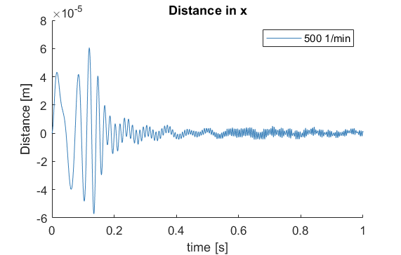
This is a Simulation file for an investigation (approximation with spring-damper elements) of a real AMB test rig (MBTR). Of interest is the behaviour of the rotor in steady state (Modal analysis) and in motion (Campbell analysis) as well as the Stationary time behaviour (at 500 rpm) under the influence of an external excitation.
Closing of all previous figures and cleaning of the workspace:
1close all
2clear all
3%clc
Import of the file path and the corresponding Configuration file:
1%% Import and formating of the figures
2
3import AMrotorSIM.* % path
4Config_Sim_eingebaut % corresponding cnfg-file
5
6Janitor = AMrotorTools.PlotJanitor(); % Instantiation of class PlotJanitor
7Janitor.setLayout(2,3); % Setting layout of the figures
Assembly and visualization of the model:
Note
The assembly of the model is the most important part of the Simulation file and must be done before the analyses.
1%% Assembly of the rotordynamic model
2
3r=Rotorsystem(cnfg,'MBTR-TestRig'); % Instantiation of class Rotorsystem
4r.assemble; % Assembly of the model parts, considering the ...
5 % components (sensors,..) from the cnfg-file
6r.rotor.assemble_fem; % Assembly of the global system matrices: M, D, G, K
7
8%% Visualization of the assembled rotor model
9
10r.show; % lists the associated components of the model in teh Matlab ...
11 % Command Window
12
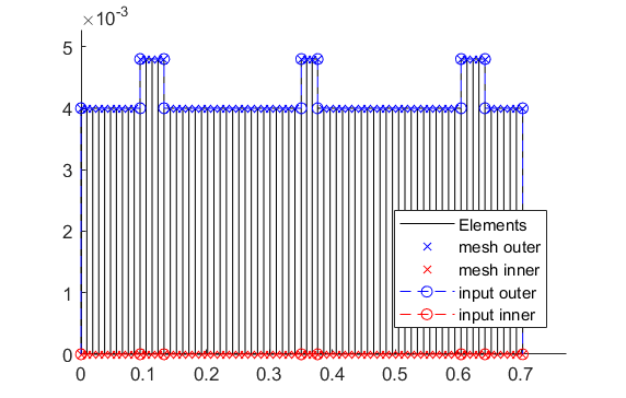
13r.rotor.show_2D(); % Plot of a side view of the rotor elements
14% r.rotor.geometry.show_2D(); % Plot of a side view of the ..
15 % rotor radii
16% r.rotor.geometry.show_3D(); % Plot of a 3D-isometry of the rotor
17% r.rotor.mesh.show_2D();
18% r.rotor.mesh.show_2D_nodes();
19% r.rotor.mesh.show_3D();
20
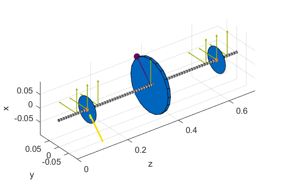
21g=Graphs.Visu_Rotorsystem(r); % Instantiation of class Visu_Rotorsystem
22g.show(); % Plot of a 3D-isometry of the rotor with sensors, loads,...
23
24u_trans_rigid_body = r.compute_translational_rigid_body_modes; % Locates ..
25 % the translational DoF's of the rotor in a matrix
26overall_mass = r.check_overall_translational_mass(u_trans_rigid_body) % ...
27 % Calculates the translational mass
2D side view of the rotor (left) and 3D isometry (right):
Note
The diameter steps in the rotor geometry (in the 2D side view) represent the reinforcements (check Configuration file for the MBTR) of the main rotor and not the disc component as seen in the 3D isometry.
Execution of the intended system analysis methods (Modal analysis and Campbell analysis) with visualization:
1%% Running system analyses
2%% Modal analysis
3
4m=Experiments.Modalanalyse(r); % Instantiation of ...
5 % class Modalanalyse
6
7rpmModalAnalysis=0;
8m.calculate_rotorsystem(16,rpmModalAnalysis);
9%
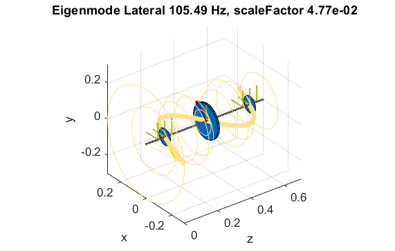
10esf= Graphs.Eigenschwingformen(m);
11esf.print_frequencies();
12esf.plot_displacements(); % Plots the 2D mode shapes
13% esf.set_plots('half','Overlay') % Plots of the odd-numbered eigenmodes ..
14 % in overlay with the original rotor
15esf.set_plots(10,'Overlay','Skip',5,'tangentialPoints',30,'scale',3) % ...
16 % Plot of the 3D mode shapes
17Janitor.cleanFigures(); % Formatting of the figures
18
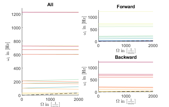
19%% Campbell analysis
20
21cmp = Experiments.Campbell(r); % Instantiation of ...
22 % class Campbell
23cmp.set_up(0:2e2:2e3,20); % Set_up (omega range in 1/min, #modes)
24cmp.calculate(); % Calculation
25
26cmpDiagramm = Graphs.Campbell(cmp); % Instantiation of ...
27 % class Campbell for figures
28cmpDiagramm.print_damping_zero_crossing(); % Prints in the Command Window
29cmpDiagramm.print_critical_speeds() % Prints in the Command Window
30cmpDiagramm.set_plots('all'); % Figures
31Janitor.cleanFigures(); % Formatting of the figures
Representation of the 10th eigenmode (upscaled and with orbits) (left) and the Campbell diagram (right) of the rotor:
Execution of time integration (at 500 rpm for 1 second) with unbalance and external excitation (Forward-whirl-sweep-force) with visualization:
 1%% Running Time Simulation
 2%% Stationary with avaliable calculation methods
 3
 4St_Lsg = Experiments.Stationaere_Lsg(r,[500],[0:0.001:0.025]); % In...
 5    %stantiation of class Stationaere_Lsg
 6
 7St_Lsg.compute_ode15s_ss; % ode15s - method
 8%St_Lsg.compute_euler_ss; % Forward euler - method (in progress)
 9%St_Lsg.compute_newmark; % newmark - method
10%St_Lsg.compute_sys_ss_variant; state space method(in progress)
11
12%% Export and visualization of the results
13%% Export
14
15d = Dataoutput.TimeDataOutput(St_Lsg); % Instantiation of class ...
16                                       % TimeDataOutput
17dataset_modalanalysis = d.compose_data(); % container: rpm ->
18                                          % (n,t,allsensorsxy)
19d.save_data(dataset_modalanalysis,'jm_whirling-chirp_500rpm');
20
21%% Visualizing results
22
23t = Graphs.TimeSignal(r, St_Lsg); % Instantiation of class TimeSignal
24o = Graphs.Orbitdarstellung(r, St_Lsg); % Instantiation of class ...
25                                     % Orbitdarstellung
26f = Graphs.Fourierdarstellung(r, St_Lsg); % Instantiation of class ...
27                                       % Fourierdarstellung
28fo = Graphs.Fourierorbitdarstellung(r, St_Lsg); % Instantiation of class ..
29                                             % Fourierorbitdarstellung
30w = Graphs.Waterfalldiagramm(r, St_Lsg); % Instantiation of class ...
31                                      % Waterfalldiagramm
32w2 = Graphs.WaterfalldiagrammTwoSided(r, St_Lsg); % Instantiation of ...
33                                       % class WaterfalldiagrammTwoSided
34
35 for sensor = r.sensors % Loop over all sensors for plotting
36          t.plot(sensor); % Time signal
37          o.plot(sensor); % Orbits
38          f.plot(sensor); % Fourier
39          fo.plot(sensor,1); % Fourierorbit 1st order
40          fo.plot(sensor,2); % Fourierorbit 2nd order
41          w.plot(sensor); % Waterfall
42          w2.plot(sensor); % Waterfall 2sided
43         Janitor.cleanFigures(); % Formatting of the figures
44 end
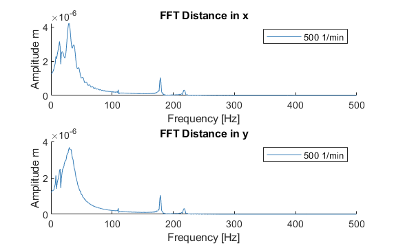
Time signal (x-direction) of the eddy-current sensor on the left side AMB (left) and the corresponding Fourier analysis (right):