Laval_Time
Config_file_LavalTime
This is a working example code for a Configuration file of a simple Laval rotor. The focus of the subsequent simulation is a Stationary time integration, a Run-up time integration and the determinationof frequency response functions (FRF’s) from the sensor time signals. The scope of the simulation can have effects on the configuration file. All code snippets can be copied and pasted into a Matlab script in the given order (recommended) and executed directly.
The first step is to define the rotor/shaft. This definition can be divided into three parts: Definition of the material parameters, the geometry of the rotor and the properties of the mesh.
 1%% Building of the rotor struct
 2cnfg.cnfg_rotor.name = 'Simple example: Laval-Rotor';
 3% All units in SI
 4cnfg.cnfg_rotor.material.name = 'steel';
 5cnfg.cnfg_rotor.material.e_module = 211e9;  %[N/m^2]
 6cnfg.cnfg_rotor.material.density  = 7860;   %[kg/m^3]
 7cnfg.cnfg_rotor.material.poisson  = 0.3;    %[-]
 8% Rayleigh damping: D=alpha1*K + alpha2*M
 9cnfg.cnfg_rotor.material.damping.rayleigh_alpha1= 1e-5;
10cnfg.cnfg_rotor.material.damping.rayleigh_alpha2= 10;
11
12%% Rotor Config
13rW = 10e-3; % Radius of the shaft [m]
14rS = 50e-3; % Radius of the disc [m]
15% Format of the geometry definition: {[z, r_outer, r_inner], ...} without..
16% start- and end-node
17cnfg.cnfg_rotor.geo_nodes = {[0 rW 0], [0.220 rW 0], [0.220 rS 0], ...
18    [0.280 rS 0], [0.280 rW 0], [0.500 rW 0]};
19clear rW rS
20
21
22%% FEM Config
23cnfg.cnfg_rotor.mesh_opt.name = 'Mesh 1';
24% Number of refinement steps between d_min and d_max
25cnfg.cnfg_rotor.mesh_opt.n_refinement = 10;
26cnfg.cnfg_rotor.mesh_opt.d_min = 0.001;
27cnfg.cnfg_rotor.mesh_opt.d_max = 0.05;
28% Definition of the element radius, if the geometry radius is not ...
29% constant in this section. Options: symmetric, mean, upper sum, lower sum
30cnfg.cnfg_rotor.mesh_opt.approx = 'symmetric';
31
The inclusion of sensors consists of the initialization of a sensor field in the cnfg-struct and a control variable called “count”. Each additional sensor (regardless of type) increases the count variable and is defined by a name, the position along the z-axis of the rotor, the sensor type and additional parameters depending on the sensor.
 1%% Initialization of the sensor section in the struct
 2cnfg.cnfg_sensor=[];
 3count = 0;
 4
 5% count = count + 1;
 6% cnfg.cnfg_sensor(count).name = 'DisplBearing1';
 7% cnfg.cnfg_sensor(count).position=0e-3; % [m]
 8% cnfg.cnfg_sensor(count).type='Displacementsensor';
 9
10count = count + 1;
11cnfg.cnfg_sensor(count).name='DisplDiscCenter';
12cnfg.cnfg_sensor(count).position=250e-3; % [m]
13cnfg.cnfg_sensor(count).type='Displacementsensor';
14
15count = count + 1;
16cnfg.cnfg_sensor(count).name='AngleDiscSensor';
17cnfg.cnfg_sensor(count).position=250e-3; % [m]
18cnfg.cnfg_sensor(count).type='Anglesensor';
19
20count = count + 1;
21cnfg.cnfg_sensor(count).name='AngleVelocDiscCenter';
22cnfg.cnfg_sensor(count).position=250e-3; % [m]
23cnfg.cnfg_sensor(count).type='AngularVelocitysensor';
24
25% count = count + 1;
26% cnfg.cnfg_sensor(count).name='DisplBearing2';
27% cnfg.cnfg_sensor(count).position=500e-3; % [m]
28% cnfg.cnfg_sensor(count).type='Displacementsensor';
29
30count = count + 1;
31cnfg.cnfg_sensor(count).name='VelocDiscCenter';
32cnfg.cnfg_sensor(count).position=250e-3; % [m]
33cnfg.cnfg_sensor(count).type='Velocitysensor';
34
35count = count + 1;
36cnfg.cnfg_sensor(count).name='AccelDiscCenter';
37cnfg.cnfg_sensor(count).position=250e-3; % [m]
38cnfg.cnfg_sensor(count).type='Accelerationsensor';
39
40count = count + 1;
41cnfg.cnfg_sensor(count).name='ForceDiscCenter';
42cnfg.cnfg_sensor(count).position=250e-3; % [m]
43cnfg.cnfg_sensor(count).type='ForceLoadPostSensor';
44
45% count = count + 1;
46% cnfg.cnfg_sensor(count).name='ForcePerturb';
47% cnfg.cnfg_sensor(count).position=100e-3; % [m]
48% cnfg.cnfg_sensor(count).type='ForceLoadPostSensor';
49%
50% count = count + 1;
51% cnfg.cnfg_sensor(count).name='ForceBearing1';
52% cnfg.cnfg_sensor(count).position=0e-3; % [m]
53% cnfg.cnfg_sensor(count).type='BearingForceSensor';
The inclusion of components (in this case bearings) consists of the initialization of a component field in the cnfg-struct and a control variable called “count”. Each additional component (regardless of type) increases the count variable and is defined by a name, the position along the z-axis of the rotor, the component type and additional parameters depending on the component.
 1%% Initialization of the components section in the struct
 2count = 0;
 3cnfg.cnfg_component = [];
 4
 5%% Bearings
 6count = count + 1;
 7cnfg.cnfg_component(count).name = 'AxBearingLeft';
 8cnfg.cnfg_component(count).type='Bearings';
 9cnfg.cnfg_component(count).subtype='SimpleAxialBearing';
10cnfg.cnfg_component(count).position=500e-3; % [m]
11cnfg.cnfg_component(count).stiffness=1e6; % [N/m]
12cnfg.cnfg_component(count).damping = 0;
13
14count = count + 1;
15cnfg.cnfg_component(count).name = 'TorqueBearingLeft';
16cnfg.cnfg_component(count).type='Bearings';
17cnfg.cnfg_component(count).subtype='SimpleTorqueBearing';
18cnfg.cnfg_component(count).position=0e-3; % [m]
19cnfg.cnfg_component(count).stiffness=1e6; % [N/m]
20cnfg.cnfg_component(count).damping = 0;
21
22count = count + 1;
23cnfg.cnfg_component(count).name = 'IsotropBearing1';
24cnfg.cnfg_component(count).type='Bearings';
25cnfg.cnfg_component(count).subtype='SimpleBearing';
26cnfg.cnfg_component(count).position=0e-3; % [m]
27cnfg.cnfg_component(count).stiffness=1e6; % [N/m]
28cnfg.cnfg_component(count).damping = 0; % [Ns/m]
29
30count = count + 1;
31cnfg.cnfg_component(count).name = 'IsotropBearing2';
32cnfg.cnfg_component(count).type='Bearings';
33cnfg.cnfg_component(count).subtype='SimpleBearing';
34cnfg.cnfg_component(count).position=500e-3; % [m]
35cnfg.cnfg_component(count).stiffness=1e6; % [N/m]
36cnfg.cnfg_component(count).damping = 0; % [Ns/m]
37
38% count = count+1;
39% cnfg.cnfg_component(count).name = 'Rigid clamping';
40% cnfg.cnfg_component(count).position=0e-3; % [m]
41% cnfg.cnfg_component(count).type='RestrictAllDofsBearing';
42% cnfg.cnfg_component(count).stiffness=1e10; % [N/m]
43% cnfg.cnfg_component(count).damping = 0;
The inclusion of loads consists of the initialization of a load field in the cnfg-struct and a control variable called “count”. Each additional load (regardless of type) increases the count variable and is defined by a name, the position along the z-axis of the rotor, the load type and additional parameters depending on the load.
  1%% Initialization of the load section in the struct
  2cnfg.cnfg_load=[];
  3count = 0;
  4
  5% % Force in constant direction
  6% count = count + 1;
  7% cnfg.cnfg_load(count).name='ConstForce';
  8% cnfg.cnfg_load(count).position=250e-3;
  9% cnfg.cnfg_load(count).betrag_x= 10;
 10% cnfg.cnfg_load(count).betrag_y= 0;
 11% cnfg.cnfg_load(count).type='Force_constant_fix';
 12
 13% Unbalance
 14count = count + 1;
 15cnfg.cnfg_load(count).name = 'SmallUnbalance';
 16cnfg.cnfg_load(count).position = 250e-3;
 17cnfg.cnfg_load(count).betrag = 1;
 18cnfg.cnfg_load(count).winkellage = 30/180*pi; % angle
 19cnfg.cnfg_load(count).width = 10e-3;
 20cnfg.cnfg_load(count).length = 70e-3;
 21cnfg.cnfg_load(count).type='Unbalance_static';
 22
 23% % Sinusoidal excitation force
 24% count = count + 1;
 25% cnfg.cnfg_load(count).name='SinForce';
 26% cnfg.cnfg_load(count).position=250e-3;
 27% cnfg.cnfg_load(count).betrag_x= 100;
 28% cnfg.cnfg_load(count).frequency_x= 50; % [Hz]
 29% cnfg.cnfg_load(count).betrag_y= 0;
 30% cnfg.cnfg_load(count).frequency_y= 50;
 31% cnfg.cnfg_load(count).type='Force_timevariant_fix';
 32
 33% % Whirl excitation force
 34% count = count + 1;
 35% cnfg.cnfg_load(count).name='WhirlForce';
 36% cnfg.cnfg_load(count).position=250e-3;
 37% cnfg.cnfg_load(count).t_start = 0; % start time [s]
 38% cnfg.cnfg_load(count).t_end = 10; % end time [s]
 39% cnfg.cnfg_load(count).betrag_x= 10;
 40% cnfg.cnfg_load(count).betrag_y= 10;
 41% cnfg.cnfg_load(count).frequency= 20; % [Hz]
 42% cnfg.cnfg_load(count).type='Force_timevariant_whirl_fwd';
 43
 44% % Chirp, Sinus sweep force
 45% count = count + 1;
 46% cnfg.cnfg_load(count).name='ChirpForce';
 47% cnfg.cnfg_load(count).position=250e-3;
 48% cnfg.cnfg_load(count).betrag_x= 1; % force amplitude x
 49% cnfg.cnfg_load(count).frequency_x_0 = 0; % start frequency x [Hz]
 50% cnfg.cnfg_load(count).frequency_x= 200; % end frequency x [Hz]
 51% cnfg.cnfg_load(count).betrag_y= 0; % force amplitude y
 52% cnfg.cnfg_load(count).frequency_y_0 = 0; % start frequency y [Hz]
 53% cnfg.cnfg_load(count).frequency_y= 0; % end frequency y [Hz]
 54% cnfg.cnfg_load(count).t_start= 0; % start time [s]
 55% cnfg.cnfg_load(count).t_end= 0.5; % end time [s]
 56% cnfg.cnfg_load(count).type='Force_timevariant_chirp';
 57
 58% % Chirp, Sinus sweep force
 59% count = count + 1;
 60% cnfg.cnfg_load(count).name='ChirpForce';
 61% cnfg.cnfg_load(count).position=250e-3;
 62% cnfg.cnfg_load(count).betrag_x= 1; % force amplitude x
 63% cnfg.cnfg_load(count).frequency_x_0 = 0; % start frequency x [Hz]
 64% cnfg.cnfg_load(count).frequency_x= 200; % end frequency x [Hz]
 65% cnfg.cnfg_load(count).betrag_y= 0; % force amplitude y
 66% cnfg.cnfg_load(count).frequency_y_0 = 0; % start frequency y [Hz]
 67% cnfg.cnfg_load(count).frequency_y= 0; % end frequency y [Hz]
 68% cnfg.cnfg_load(count).t_start= 0.5; % start time [s]
 69% cnfg.cnfg_load(count).t_end= 1; % end time [s]
 70% cnfg.cnfg_load(count).type='Force_timevariant_chirp';
 71
 72% % Chirp, Sinus sweep force
 73% count = count + 1;
 74% cnfg.cnfg_load(count).name='ChirpForce';
 75% cnfg.cnfg_load(count).position=0e-3;
 76% cnfg.cnfg_load(count).betrag_x= 0.1; % force amplitude x
 77% cnfg.cnfg_load(count).frequency_x_0 = 400; % start frequency x [Hz]
 78% cnfg.cnfg_load(count).frequency_x= 500; % end frequency x [Hz]
 79% cnfg.cnfg_load(count).betrag_y= 0; % force amplitude y
 80% cnfg.cnfg_load(count).frequency_y_0 = 0; % start frequency y [Hz]
 81% cnfg.cnfg_load(count).frequency_y= 0; % end frequency y [Hz]
 82% cnfg.cnfg_load(count).t_start= 0; start time [s]
 83% cnfg.cnfg_load(count).t_end= 1; end time [s]
 84% cnfg.cnfg_load(count).type='Force_timevariant_chirp';
 85
 86% % Forward whirl sweep force
 87% count = count + 1;
 88% cnfg.cnfg_load(count).name='FwdWhirlSweepForce';
 89% cnfg.cnfg_load(count).position=100e-3;
 90% cnfg.cnfg_load(count).betrag_x= 0.2; % force amplitude x
 91% cnfg.cnfg_load(count).betrag_y= cnfg.cnfg_load(count).betrag_x;; % force ...
 92                                                            % amplitude y
 93% cnfg.cnfg_load(count).frequency_0 = 0; % start frequency [Hz]
 94% cnfg.cnfg_load(count).frequency= 200; % end frequency [Hz]
 95% cnfg.cnfg_load(count).t_start= 0.45; % start time [s]
 96% cnfg.cnfg_load(count).t_end= 0.5; % end time [s]
 97% cnfg.cnfg_load(count).type='Force_timevariant_whirl_fwd_sweep';
 98
 99% % Backward whirl sweep force
100% count = count + 1;
101% cnfg.cnfg_load(count).name='BwdWhirlSweepKraft';
102% cnfg.cnfg_load(count).position=pos.ML1;
103% cnfg.cnfg_load(count).betrag_x= 10;
104% cnfg.cnfg_load(count).betrag_y= cnfg.cnfg_load(count).betrag_x;
105% cnfg.cnfg_load(count).frequency_0 = 0; % start frequency [Hz]
106% cnfg.cnfg_load(count).frequency= 200; % end frequency [Hz]
107% cnfg.cnfg_load(count).t_start= 0.5; % start time [s]
108% cnfg.cnfg_load(count).t_end= 1.0; % end time [s]
109% cnfg.cnfg_load(count).type='Force_timevariant_whirl_bwd_sweep';
110
111% % Muszynska-Seal laminar
112% count = count + 1;
113% cnfg.cnfg_load(count).name = 'MuszynskaSealMittig';
114% cnfg.cnfg_load(count).position=pos.DicMitte; % [m]
115% cnfg.cnfg_load(count).type='MuszynskaLaminarSeal';
116% cnfg.cnfg_load(count).sealModel = load_seal_model('Inputfiles/ ...
117%                                               TestRigNeu1.m');
118
119% % Lim-Singh-bearing
120% count = count + 1;
121% cnfg.cnfg_load(count).name = 'LimSingh1';
122% cnfg.cnfg_load(count).position=pos.Lag1; % [m]
123% cnfg.cnfg_load(count).type='LimSinghBearing';
124% cnfg.cnfg_load(count).par = load_bearing_LimSingh('Inputfiles/ ...
125%                                               parametersGupta20mm.m');
126
127% % Lim-Singh-bearing
128% count = count + 1;
129% cnfg.cnfg_load(count).name = 'LimSingh2';
130% cnfg.cnfg_load(count).position=pos.Lag2; % [m]
131% cnfg.cnfg_load(count).type='LimSinghBearing';
132% cnfg.cnfg_load(count).par = load_bearing_LimSingh('Inputfiles/ ...
133%                                               parametersGupta20mm.m');
Since no AMB’s are intended for this model, no pidControllers are needed. Nevertheless the initialization of the pidController is necessary to avoid errors. The initialization consists of the assignment of a pidController field in the cnfg-struct and the definition of a control variable “count”.
1%% Initialization of the pid-controller section in the struct
2cnfg.cnfg_pid_controller=[];
3count = 0;
No active magnetic bearings (AMB’s) are intended for this model. Nevertheless the initialization of the AMB is necessary to avoid errors. The initialization consists of the assignment of a AMB field in the cnfg-struct and the definition of a control variable “count”.
1%% Initialization of the active magnetic bearing section in the struct
2cnfg.cnfg_activeMagneticBearing = [];
3count = 0;
Simulation_file_LavalTime
This is an example code for a working Simulation file of a simple Laval rotor for time integration (Stationary and Run-up). All code snippets can be copied and pasted into a Matlab script in the given order (recommended) and executed directly.
Closing of all previous figures and cleaning of the workspace:
1close all
2clear all
3% clc
Import of the file path and the corresponding Configuration file:
1%% Import and formating of the figures
2
3import AMrotorSIM.* % path
4Config_Sim_Time % corresponding cnfg-file
5
6Janitor = AMrotorTools.PlotJanitor(); % Instantiation of class PlotJanitor
7Janitor.setLayout(2,3); %Setting layout of the figures
Assembly and visualization of the model:
Note
The assembly of the model is the most important part of the Simulation file and must be done before the analyses.
 1%% Assembly of the rotordynamic model
 2
 3r=Rotorsystem(cnfg,'Laval-Rotor'); % Instantiation of class Rotorsystem
 4r.assemble; % Assembly of the model parts, considering the ...
 5            % components (sensors,..) from the cnfg-file
 6r.rotor.assemble_fem; % Assembly of the global system matrices: M, D, G, K
 7
 8%% Visualization of the assembled rotor model
 9
10r.show; % lists the associated components of the model in teh Matlab ...
11        % Command Window
12
13r.rotor.show_2D(); % Plot of a side view of the rotor elements
14% r.rotor.geometry.show_2D();  % Plot of a side view of the ..
15                               % rotor radii
16% r.rotor.geometry.show_3D(); % Plot of a 3D-isometry of the rotor
17% r.rotor.mesh.show_2D();
18% r.rotor.mesh.show_2D_nodes();
19% r.rotor.mesh.show_3D();
20
21g=Graphs.Visu_Rotorsystem(r); % Instantiation of class Visu_Rotorsystem
22g.show(); % Plot of a 3D-isometry of the rotor with sensors, loads,...
2D side view of the rotor (left) and 3D isometry (right):


Execution of the intended analysis methods (Stationary time integration, Run-up time integration, FRF from time signals). Some are commented out:
1%% Running Time Simulation
2%% Stationary with avaliable calculation methods
3
4St_Lsg = Experiments.Stationaere_Lsg(r,[1000,1200],(0:0.001:0.02)); % In...
5 %stantiation of class Stationaere_Lsg
6
7St_Lsg.compute_ode15s_ss; % ode15s - method
8% St_Lsg.compute_euler_ss; % Forward euler - method (in progress)
9% St_Lsg.compute_newmark; % newmark - method
10% options.adapt=true; options.locTolUpper=1e-3;
11% options.locTolLower=1e-4; options.globTol=1;
12% St_Lsg.compute_newmark(options); % newmark - method with options
13% St_Lsg.compute_sys_ss_variant; (in progress)
14
15%% Run up with avaliable calculation methods
16
17% Runup = Experiments.Hochlaufanalyse(r,[0,1e3],(0:0.001:0.5)); % In...
18 %stantiation of class Stationaere_Lsg
19
20% Runup.compute_ode15s_ss; % ode15s - method
21
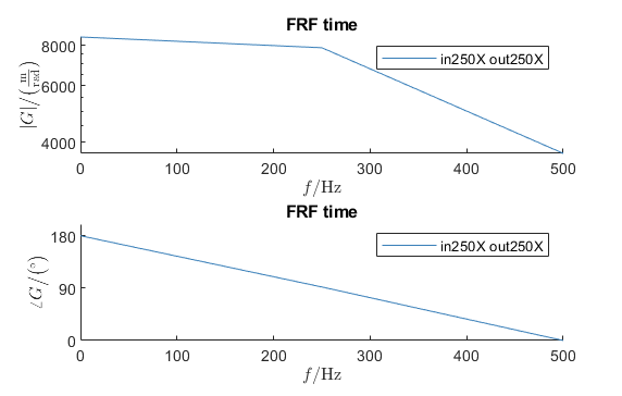
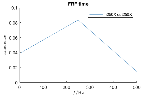
22%% FRF over time
23
24frf = Experiments.FrequenzgangfunktionTime(St_Lsg,'FRF time'); % Instantiation ...
25 % of class FrequenzgangfunktionTime
26
27frf.calculate(r.sensors(2),r.sensors(1),[1000],'u_x','u_x',4,'boxcar'); % .
28 % Calculation
Export and visualization of the results:
1%% Export and visualization of the results
2%% Export
3
4d = Dataoutput.TimeDataOutput(St_Lsg); % Instantiation of class ...
5 % TimeDataOutput
6% d = Dataoutput.TimeDataOutput(Runup);% Instantiation of class ...
7 % TimeDataOutput
8
9% dataset_modalanalysis = d.compose_data(); % container: rpm ->
10% % (n,t,allsensorsxy)
11% d.save_data(dataset_modalanalysis,'Hochlauf_Laval_U_x_sweep0_200Hz_3000rpm');
12% dataset_modalanalysis = d.compose_data_sensor_wise(); % container: rpm ->
13% % (sensor1,sensor2,.)
14% struct = d.convert_data_to_struct_sensor_wise(dataset_modalanalysis);
15% d.save_data(struct,'Hochlauf_Laval_U_x_sweep0_200Hz_3000rpm');
16
17%% Visualizing results
18
19Lsg=St_Lsg; % Lsg=Runup;
20
21t = Graphs.TimeSignal(r, Lsg); % Instantiation of class TimeSignal
22o = Graphs.Orbitdarstellung(r, Lsg); % Instantiation of class ...
23 % Orbitdarstellung
24f = Graphs.Fourierdarstellung(r, Lsg); % Instantiation of class ...
25 % Fourierdarstellung
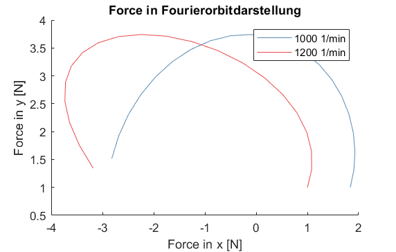
26fo = Graphs.Fourierorbitdarstellung(r, Lsg); % Instantiation of class ...
27 % Fourierorbitdarstellung
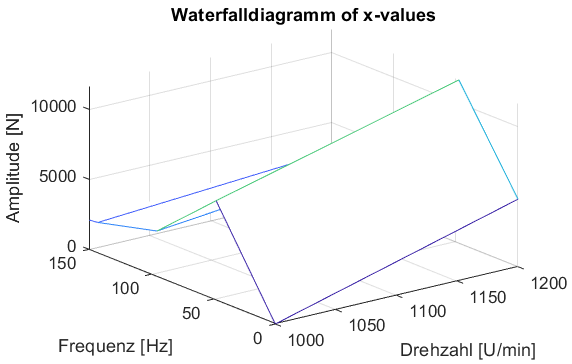
28w = Graphs.Waterfalldiagramm(r, Lsg); % Instantiation of class ...
29 % Waterfalldiagramm
30w2 = Graphs.WaterfalldiagrammTwoSided(r, Lsg); % Instantiation of class ...
31 % WaterfalldiagrammTwoSided
32
33visufrf = Graphs.Frequenzgangfunktion(frf); % Instantiation of class ...
34 % Frequenzgangfunktion for visualization
35visufrf.set_plots('bode','log','deg','coh'); % Figures
36Janitor.cleanFigures(); % Formatting of the figures
37
38 for sensor = r.sensors % Loop over all sensors for plotting
39 t.plot(sensor,[1,2,3]); % Time signal
40 o.plot(sensor); % Orbits
41 f.plot(sensor); % Fourier
42 fo.plot(sensor,1); % Fourierorbit 1st order
43 fo.plot(sensor,2); % Fourierorbit 2nd order
44 w.plot(sensor); % Waterfall
45 w2.plot(sensor); % Waterfall 2sided
46 Janitor.cleanFigures(); % Formatting of the figures
47 end
The results of the analyses performed include the following figures: