Laval_Modal
Config_file_LavalModal
This is a working example code for a Configuration file of a simple Laval rotor. The focus of the subsequent simulation is a Modal analysis, a Campbell analysis and the determination of frequency response functions (FRF’s) from the system matrices. The scope of the simulation can have effects on the configuration file. All code snippets can be copied and pasted into a Matlab script in the given order (recommended) and executed directly.
The first step is to define the rotor/shaft. This definition can be divided into three parts: Definition of the material parameters, the geometry of the rotor and the properties of the mesh:
 1%% Building of the rotor struct
 2cnfg.cnfg_rotor.name = 'Simple example: Laval-Rotor';
 3% All units in SI
 4cnfg.cnfg_rotor.material.name = 'steel';
 5cnfg.cnfg_rotor.material.e_module = 211e9;  %[N/m^2]
 6cnfg.cnfg_rotor.material.density  = 7860;   %[kg/m^3]
 7cnfg.cnfg_rotor.material.poisson  = 0.3;    %[-]
 8% Rayleigh damping: D=alpha1*K + alpha2*M
 9cnfg.cnfg_rotor.material.damping.rayleigh_alpha1= 1e-5;
10cnfg.cnfg_rotor.material.damping.rayleigh_alpha2= 10;
11
12%% Rotor Config
13rW = 10e-3; % Radius of the shaft [m]
14rS = 50e-3; % Radius of the disc [m]
15% Format of the geometry definition: {[z, r_outer, r_inner], ...} without..
16% start- and end-node:
17cnfg.cnfg_rotor.geo_nodes = {[0 rW 0], [0.220 rW 0], [0.220 rS 0], ...
18    [0.280 rS 0], [0.280 rW 0], [0.500 rW 0]};
19clear rW rS
20
21
22%% FEM Config
23cnfg.cnfg_rotor.mesh_opt.name = 'Mesh 1';
24% Number of refinement steps between d_min and d_max:
25cnfg.cnfg_rotor.mesh_opt.n_refinement = 10;
26cnfg.cnfg_rotor.mesh_opt.d_min = 0.001;
27cnfg.cnfg_rotor.mesh_opt.d_max = 0.05;
28% Definition of the element radius, if the geometry radius is not ...
29% constant in this section. Options: symmetric, mean, upper sum, lower sum:
30cnfg.cnfg_rotor.mesh_opt.approx = 'symmetric';
31
Sensors are not absolutely necessary for the desired analysis methods, so that no sensors need to be defined. Nevertheless the initialization of the sensor is necessary to avoid errors. The initialization consists of the assignment of a sensor field in the cnfg-struct and the definition of a control variable “count”:
1%% Initialization of the sensor section in the struct
2cnfg.cnfg_sensor=[];
3count = 0;
The inclusion of components (in this case bearings) consists of the initialization of a component field in the cnfg-struct and a control variable called “count”. Each additional component (regardless of type) increases the count variable and is defined by a name, the position along the z-axis of the rotor, the component type and additional parameters depending on the component:
 1%% Initiation of the components section in the struct
 2count = 0;
 3cnfg.cnfg_component = [];
 4
 5%% Bearings
 6count = count + 1;
 7cnfg.cnfg_component(count).name = 'AxBearingLeft';
 8cnfg.cnfg_component(count).type='Bearings';
 9cnfg.cnfg_component(count).subtype='SimpleAxialBearing';
10cnfg.cnfg_component(count).position=500e-3; % [m]
11cnfg.cnfg_component(count).stiffness=1e6; % [N/m]
12cnfg.cnfg_component(count).damping = 0; % [Ns/m]
13
14count = count + 1;
15cnfg.cnfg_component(count).name = 'TorqueBearingLeft';
16cnfg.cnfg_component(count).type='Bearings';
17cnfg.cnfg_component(count).subtype='SimpleTorqueBearing';
18cnfg.cnfg_component(count).position=0e-3; % [m]
19cnfg.cnfg_component(count).stiffness=1e6; % [N/m]
20cnfg.cnfg_component(count).damping = 0; % [Ns/m]
21
22count = count + 1;
23cnfg.cnfg_component(count).name = 'IsotropBearing1';
24cnfg.cnfg_component(count).type='Bearings';
25cnfg.cnfg_component(count).subtype='SimpleBearing';
26cnfg.cnfg_component(count).position=0e-3; % [m]
27cnfg.cnfg_component(count).stiffness=1e6; % [N/m]
28cnfg.cnfg_component(count).damping = 0; % [Ns/m]
29
30count = count + 1;
31cnfg.cnfg_component(count).name = 'IsotropBearing2';
32cnfg.cnfg_component(count).type='Bearings';
33cnfg.cnfg_component(count).subtype='SimpleBearing';
34cnfg.cnfg_component(count).position=500e-3; % [m]
35cnfg.cnfg_component(count).stiffness=1e6; % [N/m]
36cnfg.cnfg_component(count).damping = 0; % [Ns/m]
37
38% count = count+1;
39% cnfg.cnfg_component(count).name = 'Rigid clamping';
40% cnfg.cnfg_component(count).position=0e-3; % [m]
41% cnfg.cnfg_component(count).type='RestrictAllDofsBearing';
42% cnfg.cnfg_component(count).stiffness=1e10; % [N/m]
43% cnfg.cnfg_component(count).damping = 0;
Loads are not absolutely necessary for the desired analysis methods, so that no loads need to be defined. Nevertheless the initialization of the load is necessary to avoid errors. The initialization consists of the assignment of a load field in the cnfg-struct and the definition of a control variable “count”:
1%% Initialization of the load section in the struct
2cnfg.cnfg_load=[];
3count = 0;
Since no AMB’s are intended for this model, no pidControllers are needed. Nevertheless the initialization of the pidController is necessary to avoid errors. The initialization consists of the assignment of a pidController field in the cnfg-struct and the definition of a control variable “count”:
1%% Initialization of the pid-controller section in the struct
2cnfg.cnfg_pid_controller=[];
3count = 0;
No active magnetic bearings (AMB’s) are intended for this model. Nevertheless the initialization of the AMB is necessary to avoid errors. The initialization consists of the assignment of a AMB field in the cnfg-struct and the definition of a control variable “count”:
1%% Initialization of the active magnetic bearing section in the struct
2cnfg.cnfg_activeMagneticBearing = [];
3count = 0;
Simulation_file_LavalModal
This is an example code for a working Simulation file of a simple Laval rotor for system analyses (Campbell, Modal, FRF analyses). All code snippets can be copied and pasted into a Matlab script in the given order (recommended) and executed directly.
Closing of all previous figures and cleaning of the workspace:
1close all
2clear all
3% clc
Import the file path and the corresponding Configuration file:
1%% Import and formating of the figures
2
3import AMrotorSIM.*; % path
4Config_Sim_Modal; % corresponding cnfg-file
5
6Janitor = AMrotorTools.PlotJanitor(); % Instantiation of class PlotJanitor
7Janitor.setLayout(2,3); %Formatting of the figures
Assembly and visualization of the model:
Note
The assembly of the model is the most important part of the Simulation file and must be done before the analyses.
 1%% Assembly of the rotordynamic model
 2
 3r=Rotorsystem(cnfg,'Laval-Rotor'); % Instantiation of class Rotorsystem
 4r.assemble; % assembly of the model parts, considering the ...
 5            % components (sensors,..) from the cnfg-file
 6r.rotor.assemble_fem; % assembly of the global (rotor) system ...
 7                      % matrices: M, D, G, K
 8
 9%% Visualization of the assembled rotor model
10
11r.show; % lists the associated components of the model in teh Matlab ...
12        % Command Window
13
14r.rotor.show_2D(); % Plot of a side view of the rotor elements
15% r.rotor.geometry.show_2D();  % Plot of a side view of the ..
16                               % rotor radii
17% r.rotor.geometry.show_3D(); % Plot of a 3D-isometry of the rotor
18% r.rotor.mesh.show_2D();
19% r.rotor.mesh.show_2D_nodes();
20% r.rotor.mesh.show_3D();
21
22g=Graphs.Visu_Rotorsystem(r); % Instantiation of class Visu_Rotorsystem
23g.show(); % Plot of a 3D-isometry of the rotor with sensors, loads,...
24
25u_trans_rigid_body = r.compute_translational_rigid_body_modes; % Locates ..
26                         % the translational DoF's of the rotor in a matrix
27overall_mass = r.check_overall_translational_mass(u_trans_rigid_body) % ...
28                         % Calculates the translational mass
2D side view of the rotor (left) and 3D isometry (right):


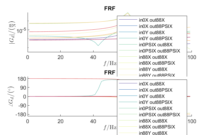
Execution of the intended analysis methods (FRF, Campbell, Modal analysis) and their visualization:
1%% Running system analyses
2%% Frequency response function
3
4frf=Experiments.Frequenzgangfunktion(r,'FRF'); % Instantiation of ...
5 % class Frequenzgangfunktion
6type = 'd'; % FRF type: displ. 'd', veloc. 'v', accel. 'a'
7inPos = [0,100,200]*1e-3; % Input positions on the rotor axis
8outPos = 100e-3; % Output positions along the rotor axis
9f = 1:2:100; % Frequency resolution of the FRF
10rpm = 0; % Rotational speed
11[f,H]=frf.calculate(f,inPos,outPos,type,rpm,{'u_x','u_y','psi_x'}, ...
12 {'u_x','psi_x'}); % Calculation of the FRF's from the three input ...
13 % directions {'u_x','u_y','psi_x'} to the two ...
14 % output directions {'u_x','psi_x'} at the ...
15 % corresponding positions
16[deltaIn,deltaOut]=frf.print_distance_delta; % Plot of the gap between ...
17 % the desired positions along the rotor axis and ...
18 % the closest node position in the Command Window.
19
20visufrf = Graphs.Frequenzgangfunktion(frf); % Instantiation of ...
21 % class Frequenzgangfunktion for figures
22visufrf.set_plots('amplitude','db') % Amplitude plot of all FRF's
23visufrf.set_plots('phase','db') % Phase plot of all FRF's
24visufrf.set_plots('bode','log','deg') % Bode plot of all FRF's
25visufrf.set_plots('nyquist') % Nyquist plot of all FRF's
26Janitor.cleanFigures(); % Formatting of the figures
27
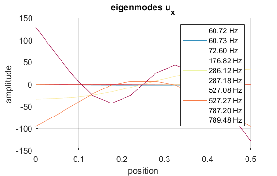
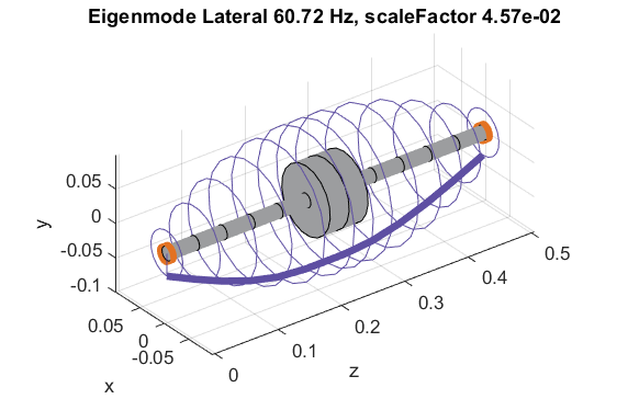
28%% Modal analysis
29
30m=Experiments.Modalanalyse(r); % Instantiation of ...
31 % class Modalanalyse
32m.calculate_rotorsystem(10,3e3); % Calcualtion (#modes,rpm)
33
34esf=Graphs.Eigenschwingformen(m); % Instantiation of ...
35 % class Eigenschwingformen
36esf.print_frequencies(); % Print of the eigenfrequencies ...
37 % with the corresponding modal damping ...
38 % in the Command Window
39esf.plot_displacements(); % Figures of the eigenmodes ...
40 % in specific directions
41esf.set_plots('half','Overlay') % Plots of the odd-numbered eigenmodes ...
42 % in overlay with the original rotor
43Janitor.cleanFigures(); % Formatting of the figures
44
45
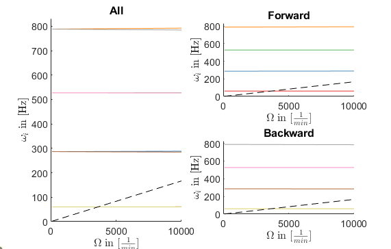
46%% Campbell diagramm
47
48cmp = Experiments.Campbell(r); % Instantiation of ...
49 % class Campbell
50cmp.set_up(1e2:1e2:10e3,8); % Set_up (omega range in 1/min, #modes)
51cmp.calculate(); % Calculation
52
53cmpDiagramm = Graphs.Campbell(cmp); % Instantiation of ...
54 % class Campbell for figures
55cmpDiagramm.print_damping_zero_crossing(); % Prints in the Command Window
56cmpDiagramm.print_critical_speeds() % Prints in the Command Window
57cmpDiagramm.set_plots('all'); % Figures
58% cmpDiagramm.set_plots('backward');
59% cmpDiagramm.set_plots('forward');
60Janitor.cleanFigures(); % Formatting of the figures
The results of the analyses performed include the following figures: